Statistics of the dynamics¶

Once qualitative intuition has been gained by plotting time series from a few samples (see Plotting samples) one can inspect quantitatively the dynamics of a dataset by using tunacell’s pre-defined tools.

Univariate and bivariate analysis tools are coded in tunacell in order to describe the statistics of single, resp. a couple of, observable(s).

We start with a background introduction to those concepts. Then we set the session, and show tunacell’s procedures.

Note

This manual page is rather tedious. To be more practical, open, read, and run the following scripts univariate-analysis.py, univariate-analysis-2.py, and bivariate-analysis.py. Background information on this page, and figures might be useful as a side help.

Background¶

We consider a stochastic process \(x(t)\).

One-point functions¶

One-point functions are statistical estimates of functions of a single time-point. Typical one-point functions are the average at a given time

\[\langle x(t) \rangle\]

where the notation \(\langle \cdot \rangle\) means taking the ensemble average of the quantity; or the variance

\[\sigma^2 (t) = \langle (x(t) - \langle x(t) \rangle )^2 \rangle\]

Inspecting these functions provides a first quantitative approach of the studied process.

In our case, time series are indexed to acquisition times \(t_i\), where \(i=0,\ 1,\ 2,\ \dots\). Usually

\[t_i = t_{\mathrm{offset}} + i \times \Delta t\]

where \(\Delta t\) is the time interval between two frame acquisitions, and \(t_{\mathrm{offset}}\) is an offset that sets the origin of times.

Then if we denote \(s^{(1)}_i\) as the number of cells acquired at time index \(i\), the average value at the same time of observable \(x\) is evaluated in tunacell as:

\[\langle x(t_i) \rangle = \frac{1}{s^{(1)}_i} \sum_{k=1}^{s^{(1)}_i} x^{(k)}(t_i)\]

where \(x^{(k)}(t)\) is the value of observable \(x\) in cell \(k\) at time \(t\).

Two-point functions¶

Two-point functions are statistical estimates of functions of two time-points. The typical two-point function is the auto-correlation function, defined as:

\[a(s, t) = \langle (x(s) - \langle x(s) \rangle) \times (x(t) - \langle x(t) \rangle) \rangle\]

In tuna it is estimated using:

\[a_{ij} = \frac{1}{s^{(2)}_{ij}} \sum_{k=1}^{s_{ij}} x^{(k)}(t_i) \times x^{(k)}(t_j) - \langle x(t_i) \rangle \langle x(t_j) \rangle \equiv a(t_i, t_j)\]

where the sum over \(k\) means over lineages connecting times \(t_i\) to \(t_j\) (there are \(s^{(2)}_{ij}\) such lineages).

With our method, for a cell living at time \(t_i\), there will be at most one associated descendant cell at time \(t_j\). There may be more descendants living at \(t_j\), but only one is picked at random according to our lineage decomposition procedure.

For identical times, the auto-correlation coefficient reduces to the variance:

\[a_{ii} \equiv \langle \left( x(t_i) - \langle x(t_i) \rangle \right)^2 \rangle = \sigma^2(t_i)\]

Under stationarity hypothesis, the auto-correlation function depends only on time differences such that:

\[a(s, t) = \tilde{a}(s-t)\]

(and the function \(\tilde{a}\) is symmetric: \(\tilde{a}(-u)=\tilde{a}(u)\)).

In tuna, there is a special procedure to estimate \(\tilde{a}\) which is to use the lineage decomposition to generate time series, and then for a given time interval \(u\), we collect all couple of points \((t_i, t_j)\) such that \(u = t_i - t_j\), and perform the average over all these samples.

We can extend such a computation to two observables \(x(t)\) and \(y(t)\). The relevant quantity is the cross-correlation function

\[c(s, t) = \langle (x(s) - \langle x(s) \rangle ) \times (y(t) - \langle y(t) \rangle ) \rangle\]

which we estimate through cross-correlation coefficients

\[c_{ij} = c(t_i, t_j)\]

Again under stationarity hypothesis, the cross-correlation function depends only on time differences:

\[c(s, t) = \tilde{c}(s - t)\]

though now the function \(\tilde{c}\) may not be symmetric.

Note

At this stage of development, extra care has not been taken to ensure ideal properties for our statistical estimates such as unbiasedness. Hence caution should be taken for the interpretation of such estimates.

Warming-up [1]¶

We start with:

from tunacell import Experiment, Observable, FilterSet
from tunacell.filters.cells import FilterCellIDparity

exp = Experiment('~/tmptunacell/simutest')

# define a condition
even = FilterCellIDparity('even')
condition = FilterSet(label='evenID', filtercell=even)

Note

The condition we are using in this example serves only as a test; we do not expect that the subgroup of cells with even identifiers differ from all cells, though we expect to halve the samples and thus we can appreciate the finite-size effects.

In this example, we look at the following dynamic observables:

ou = Observable(name='exact-growth-rate', raw='ou')

The ou—Ornstein-Uhlenbeck—observable process models instantaneous growth rate. As it is a numerical simulation, we have some knowledge of the statistics of such process. We import some of them from the metadata:

md = exp.metadata
params = md['ornstein_uhlenbeck_params']
ref_mean = params['target']
ref_var = params['noise']/(2 * params['spring'])
ref_decayrate = params['spring']

Starting with the univariate analysis¶

To investigate the statistics of a single observable over time, tuna uses the lineage decomposition to parse samples and computes incrementally one- and two-point functions.

Estimated one-point functions are the number of samples and the average value at each time-point. Estimated two-point functions are the correlation matrix between any couple of time-points, which reduces to the variance for identical times.

The module tuna.stats.api stores most of the functions to be used

To perform the computations, we import tunacell.stats.api.compute_univariate() and call it:

from tunacell.stats.api import compute_univariate
univ = compute_univariate_dynamics(exp, ou, cset=[condition, ])

This function computes one-point and two-point functions as described above and stores the results in univ, a tuna.stats.single.Univariate instance. Results are reported for the unconditioned data, under the master label, and for each of the conditions provided in the cset list. Each individual group is an instance of tuna.stats.single.UnivariateConditioned, which attributes points directly to the estimated one- and two-point functions. These items can be accessed as values of a dictionary:

result = univ['master']
result_conditioned = univ[repr(condition)]

As the master is always defined, one can alternatively use the attribute:

result = univ.master

Inspecting univariate results¶

The objects result and result_conditioned are instances of the UnivariateConditioned class, where one can find the following attributes: time, count_one, average, count_two, and autocorr; these are Numpy arrays.

To be explicit, the time array is the array of each \(t_i\) where observables have been evaluated. The count_one array stores the corresponding number of samples \(s^{(1)}_i\) (see Background), and the average array stores the \(\langle x(t_i) \rangle\) average values.

One can see an excerpt of the table of one-point functions by typing:

result.display_onepoint(10)  # 10 lines excerpt

which should be like:

   time  counts   average   std_dev
 0.0     200  0.011725  0.001101
 5.0     207  0.011770  0.001175
10.0     225  0.011780  0.001201
15.0     253  0.011766  0.001115
20.0     265  0.011694  0.001119
25.0     286  0.011635  0.001149
30.0     301  0.011627  0.001147
35.0     318  0.011592  0.001173
40.0     337  0.011564  0.001189
45.0     354  0.011578  0.001150

The count_two 2d array stores matrix elements \(s^{(2)}_{ij}\) corresponding to the number of independent lineages connecting time \(t_i\) to \(t_j\), and the attribute autocorr stores the matrix elements \(a_{ij}\) (auto-covariance coefficients). The std_dev column of the latter table is in fact computed as the square root of the diagonal of such auto-covariance matrix (such diagonal is the variance at each time-point).

An excerpt of the auto-covariance function can be printed:

result.display_twopoint(10)

which should produce something like:

   time-row  time-col  counts  autocovariance
     0.0       0.0     200    1.211721e-06
     0.0       5.0     200    1.093628e-06
     0.0      10.0     200    7.116838e-07
     0.0      15.0     200    3.415255e-07
     0.0      20.0     200    6.881773e-07
     0.0      25.0     200    1.027559e-06
     0.0      30.0     200    1.053278e-06
     0.0      35.0     200    5.925049e-07
     0.0      40.0     200   -7.884958e-08
     0.0      45.0     200   -8.413113e-08

Examples¶

To fix the idea, if we want to plot the sample average as a function of time for the whole statistical ensemble, here’s how one can do:

import matplotlib.pyplot as plt
plt.plot(univ.master.time, univ.master.average)
plt.show()

If one wants to plot the variance as a function of time for the condition results:

import numpy as np
res = univ[repr(condition)]
plt.plot(res.time, np.diag(res.autocorr))

To obtain a representation of the auto-correlation function, we set a time of reference and find the closest index in the time array:

tref = 80.
iref = np.argmin(np.abs(res.time - tref)  # index in time array
plt.plot(res.time, res.autocorr[iref, :])

Such a plot represents the autocorrelation \(a(t_{\mathrm{ref}}, t)\) as a function of \(t\).

We will see below some pre-defined plotting capabilities.

Computations can be exported as text files¶

To save the computations, just type:

univ.export_text()

This convenient function exports computations as text files, under a folder structure that stores the context of the computation such as the filter set, the various conditions that have been applied, and the different observables over which computation has been performed:

simutest/analysis/filterset/observable/condition

The advantage of such export is that it is possible to re-load parameters from an analysis in a different session.

Plotting results¶

tunacell comes with the following plotting functions:

from tunacell.plotting.dynamics import plot_onepoint, plot_two_points

that works with tuna.stats.single.Univariate instances such as our results stored in univ:

fig = plot_onepoint(univ, mean_ref=ref_mean, var_ref=ref_var, show_ci=True, save=True)

One point plots are saved in the simutest/analysis/filterset/observable folder since all conditions are represented.

The first figure, stored in fig1, looks like:

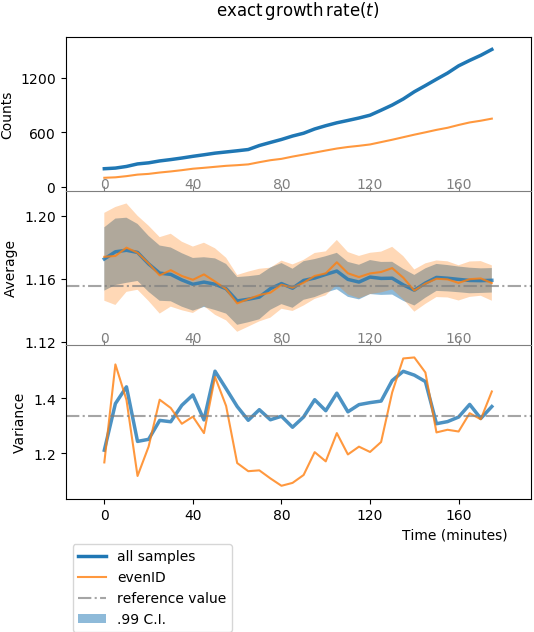
../_images/plot_onepoint_exact-growth-rate_ALL.png

Plot of one-point functions computed by tuna. The first row shows the sample counts vs. time, \(s^{(1)}_i\) vs. \(t_i\). The middle row shows the sample average \(\langle x(t_i) \rangle\) vs. time. Shadowed regions show the 99% confidence interval, computed in the large sample size limit with the empirical standard deviation. The bottom row shows the variance \(\sigma^2(t_i)\). The blue line shows results for the whole statistical ensemble, whereas the orange line shows results for the conditioned sub-population (cells with even identifier).

We can represent two point functions:

fig2 = plot_twopoints(univariate, condition_label='master', trefs=[40., 80., 150.],
                  show_exp_decay=ref_decayrate)

The second figure, stored in fig2, looks like so:

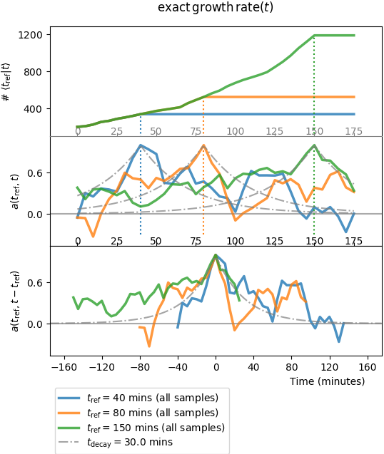
../_images/plot_twopoints_exact-growth-rate_ALL.png

Plot of two-point functions. Three times of reference are chosen to display the associated functions. Top row shows the sample counts, i.e. the number of independent lineages used in the computation that connect tref to \(t\). Middle row shows the associated auto-correlation functions \(a(t_{\mathrm{ref}}, t)/\sigma^2(t_{\mathrm{ref}})\). The bottom row show the translated functions \(a(t_{\mathrm{ref}}, t-t_{\mathrm{ref}})/\sigma^2(t_{\mathrm{ref}})\). One can guess that they peak at \(t-t_{\mathrm{ref}} \approx 0\), though decay on both sides are quite irregular compared to the expected behaviour due to the low sample size.

The view proposed on auto-correlation functions for specific times of reference is not enough to quantify the decay and associate a correlation time. A clever trick to gain statistics is to pool all data where the process is stationary and numerically evaluate \(\tilde{a}\).

Computing the auto-correlation function under stationarity¶

By inspecting the average and variance in the one-point function figure above, the user can estimate whether the process is stationary and where (over the whole time course, or just over a subset of it). The user is prompted to define regions where the studied process is (or might be) stationary. These regions are saved automatically:

# %% define region(s) for steady state analysis
# call the Regions object initialized on parser
regs = Regions(exp)
# this call reads previously defined regions, show them with
print(regs)

# then use one of the defined regions
region = regs.get('ALL')  # we take the entire time course

Computation options need to be provided. They dictate how the mean value must be substracted: either global mean over all time-points defined within a region, either locally where the time-dependent average value is used; and how segments should be sampled: disjointly or not. Default settings are set to use global mean value and disjoint segments:

# define computation options
options = CompuParams()

To compute the stationary auto-correlation function \(\tilde{a}\) use:

from tunacell.stats.api import compute_stationary
stat = compute_stationary(univ, region, options)

The first argument is the Univariate instance univ, the second argument is the time region over which to accept samples, and the third are the computation options.

Here our process is stationary by construct over the whole time period of the simulation so we choose the ‘ALL’ region. Our options is to substract the global average value for the process, and to accept only disjoint segments for a given time interval: this will ensure that samples used for a given time interval are independent (as long as the process is Markovian) and we can estimate the confidence interval by computing the standard deviation of all samples for a given time interval.

stat is an instance of tuna.stats.single.StationaryUnivariate which is structured in the same way with respect to master and conditions. Each of its items (e.g. stat.master, or stat[repr(condition)]) is an instance of tuna.stats.single.StationaryUnivariateConditioned and stores information in the following attributes:

time: the 1d array storing time interval values,
counts: the 1d array storing the corresponding sample counts,
autocorr: the 1d array storing the value of the auto-correlation function \(\tilde{a}\) for corresponding time intervals.
dataframe: a Pandas.dataframe instance that collects data points used in the computation ; each row corresponds to a single data point (in a single cell), with information on the acquisition time, the cell identifier, the value of the observable, and as many boolean columns as there are conditions, plus the master (no condition), that indicate whether a sample has been taken or not. This is a convenient dataframe to draw e.g. marginal distributions.

Plotting results¶

tunacell provides a plotting function that returns a Figure instance:

from tunacell.plotting.dynamics import plot_stationary
fig = plot_stationary(stat, show_exp_decay=ref_decayrate, save=True)

The first argument must be a tuna.stats.single.StationaryObservable instance. The second parameter displays an exponential decay (to compare with data).

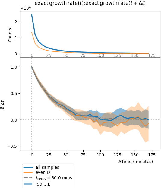
../_images/plot_stationary_exact-growth-rate_ALL.png

Plot of stationary autocorrelation function. Top row is the number of samples, i.e. the number of (disjoint) segments of size \(\Delta t\) found in the decomposed lineage time series. Middle row is the auto-correlation function \(\tilde{a}(\Delta t)/\sigma^2(0)\). Confidence intervals are computed independently for each time interval, in the large sample size limit.

Exporting results as text files¶

Again it is possible to export results as text files under the same folder structure by typing:

stat.export_text()

This will create a tab-separated text file called stationary_<region.name>.tsv that can be read with any spreadsheet reader.

In addition, the dataframe of single time point values is exported as a csv file under the filterset folder as data_<region.name>_<observable.label()>.csv.

A note on loading results¶

As described above, results can be saved in a specific folder structure that not only store the numerical results but also the context (filterset, conditions, observables, regions).

Then it is possible to load results by parsing the folder structure and reading the text files. To do so, initialize an analysis object with some settings, and try to read results from files:

from tunacell.stats.api import load_univariate
# load univariate analysis of experiment defined in parser
univ = load_univariate(exp, ou, cset=[condition, ])

The last call will work only if the analysis has been performed and exported to text files before. Hence a convenient way to work is:

try:
    univ = load_univariate(exp, ou, cset=[condition, ])
except UnivariateIOError as uerr:
    print('Impossible to load univariate {}'.format(uerr))
    print('Launching computation')
    univ = compute_univariate(exp, ou, cset=[condition, ])
    univ.export_text()

Bivariate analysis: cross-correlations¶

Key questions are to check which observables correlate, and how they correlate in time. The appropriate quantity to look at is the cross-correlation function, \(c(s, t)\), and the stationary cross-correlation funtion \(\tilde{c}(\Delta t)\) defined above (see Background).

To estimate these functions, one first need to have run the univariate analyses on the corresponding observables. We take the univariate objects corresponding to the ou and gr observables:

# local estimate of growth rate by using the differentiation of size measurement
# (the raw column 'exp_ou_int' plays the role of cell size in our simulations)
gr = Observable(name='approx-growth-rate', raw='exp_ou_int',
                differentiate=True, scale='log',
                local_fit=True, time_window=15.)
univ_gr = compute_univariate(exp, gr, [condition, ])

# import api functions
from tunacell.stats.api import (compute_bivariate,
                            compute_stationary_bivariate)
# compute cross-correlation matrix
biv = compute_cross(univ, univ_gr)
biv.export_text()

# compute cross-correlation function under stationarity hypothesis
sbiv = compute_cross_stationary(univ, univ_gr, region, options)
sbiv.export_text()

These objects again point to items corresponding to the unconditioned data and each of the conditions.

Again, cross-correlation functions as a function of two time-points (results stored in biv), the low sample size is a limit to get a smooth numerical estimate and we turn to the estimate under stationary hypothesis in order to pool all samples.

Inspecting cross-correlation results¶

We can inspect the master result:

master = biv.master

or any of the conditioned dataset:

cdt = biv[repr(condition)]

where condition is an item of each of the cset lists (one for each single object). Important attributes are:

times: a couple of lists of sequences of times, corresponding respectively to the times evaluated for each item in singles, or \(\{ \{s_i\}_i, \{t_j\}_j \}\) where \(\{s_i\}_i\) is the sequence of times where the first single item has been evaluated, and \(\{t_j\}_j\) is the sequence of times where the second single observable has been evaluated. Note that the length \((p, q)\) of these vectors may not coincide.
counts: the \((p, q)\) matrix giving for entry \((i, j)\) the number of samples in data where an independent lineage has been drawn between times \(s_i\) and \(t_j\).
corr: the \((p, q)\) matrix giving for entry \((i, j)\) the value of estimated correlation \(c_(s_i, t_j)\).

It is possible to export data in text format using:

biv.export_text()

It will create a new folder <obs1>_<obs2> under each condition folder and store the items listed above in text files.

Inspecting cross-correlation function at stationarity¶

In the same spirit:

master = sbiv.master

gets among its attributes array that stores time intervals, counts, and values for correlation as a Numpy structured array. The dataframe attribute points to a Pandas.dataframe that recapitulates single time point data in a table, with boolean columns for each condition.

It is possible to use the same plotting function used for stationary autocorrelation functions:

plot_stationary(sbiv, ref_decay=ref_decayrate)

which should plot something like:

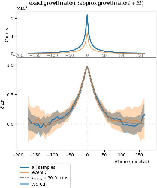
../_images/plot_stationary_exact-growth-rate---approx-growth-rate_ALL.png

Plot of the stationary cross-correlation function of the Ornstein-Uhlenbeck process with the local growth rate estimate using the exponential of the integrated process. It is symmetric and not very informative since it should more or less collapse with the auto-correlation of one of the two observables, since the second is merely a local approximation of the first.

Other examples¶

If one performs a similar analysis with the two cell-cycle observables, for example:

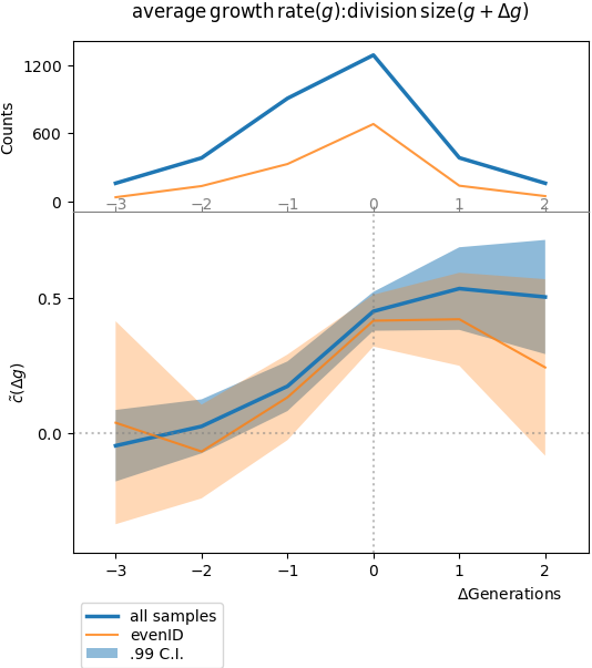
../_images/plot_stationary_average-growth-rate---division-size_ALL.png

Plot of the stationary cross-correlation function of the cell-cycle average growth rate with the cell length at division, with respect to the number of generations. We expect that a fluctuation in cell-cycle average growth rate influences length at division in the same, or in later generations. This is why we observe the highest values of correlation for \(\Delta t = 0,\ 1,\ 2\) generations, and nearly zero correlation for previous generations (there is no size control mechanism in this simulation).

Footnotes

[1]	This document has been written during Roland Garros tournament…